Linear Regression Assumptions

The linear regression is one of simplest modelling techniques that is widely used. Even though the prediction power of regression models are not as good as many of the recent machine learning techniques, it is very useful in making model interpretations - in answering questions such as which explanatory variables have the most influence on the dependent variable ($y$). Most of the time, we just dump the variables as input to the software and determine the ‘best-fit line’. As a result, we tend to ignore the underlying assumptions behind a linear regression model, some of which have consequences on the model performance. In this post, I wish to share few of the assumptions that one needs to check for while building a linear regression model. I learnt these during my course on Analytical Techniques in Transportation Engineering taught by Dr. Karthik K Srinivasan during my undergraduate studies.

1. Linear Functional Form

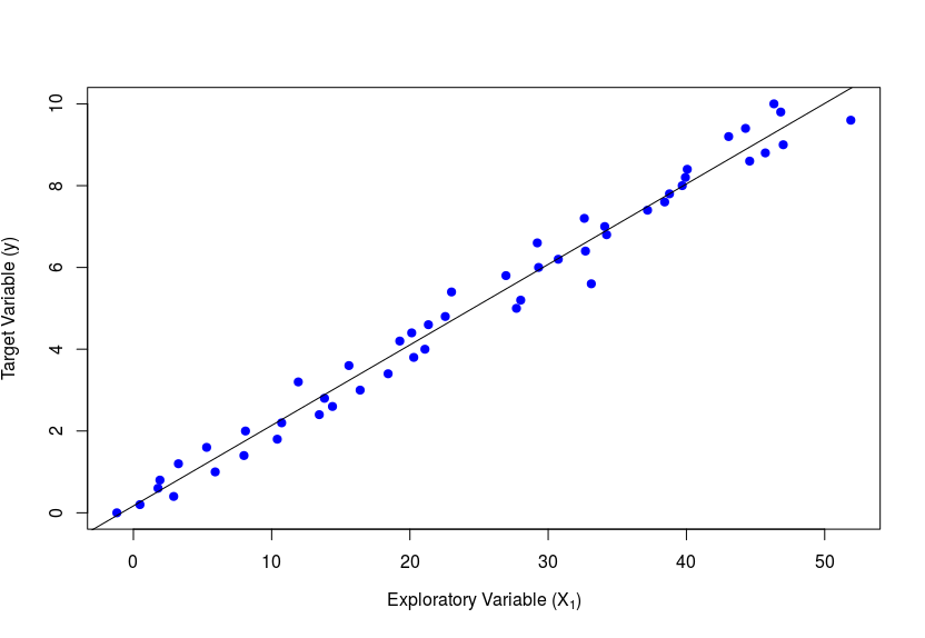
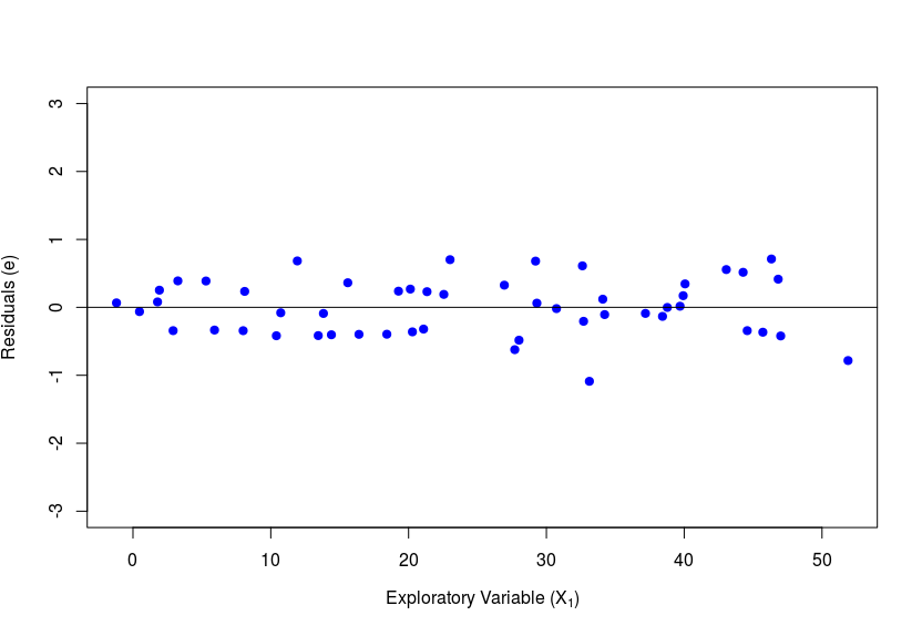
As the name rightly suggests, the y-variable is required to have a linear relationship with each of the $X_i$. We can visually check this by plotting $y$ against each $X_i$ and see if the scatter plot looks linear. Alternatively, we could also plot the residuals $e_i=(y_i-\hat{y}_i)$ on y-axis and the explanatory variables ($X_i$) on the x-axis (one at a time). If this gives a horizontal line passing through zero with no particular trend among the scatter points, then the assumption of linearity holds good. Incase the graphs do not come out as mentioned above, then it could be because of a violation of the assumption. In such a scenario the respective $X_i$ can be transformed - For example, one could use or $\sqrt{X_i}$ or $\log{X_i}$ instead of $X_i$. The figures below show the ideal graphs where this assumption holds true.

2. Constant Error Variance

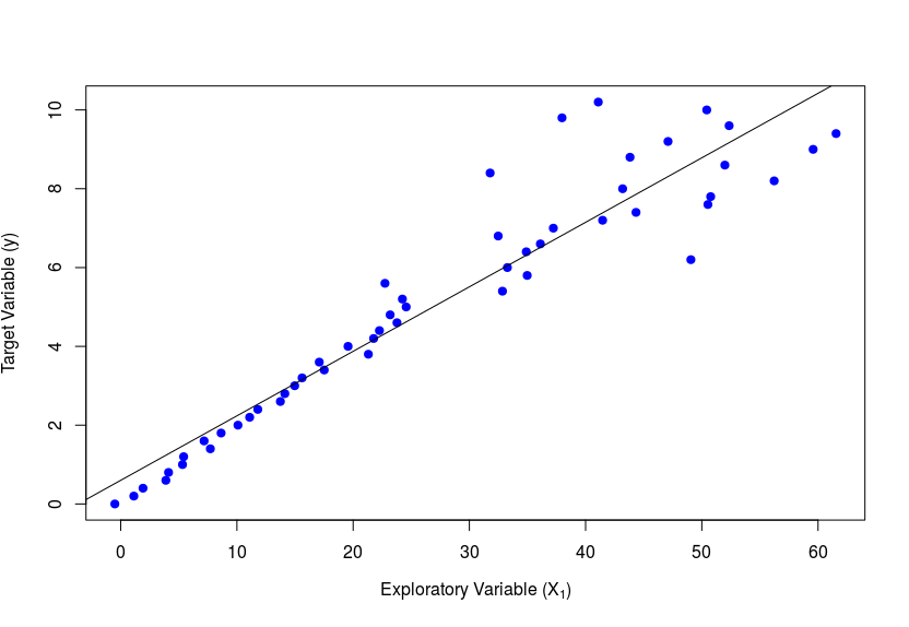
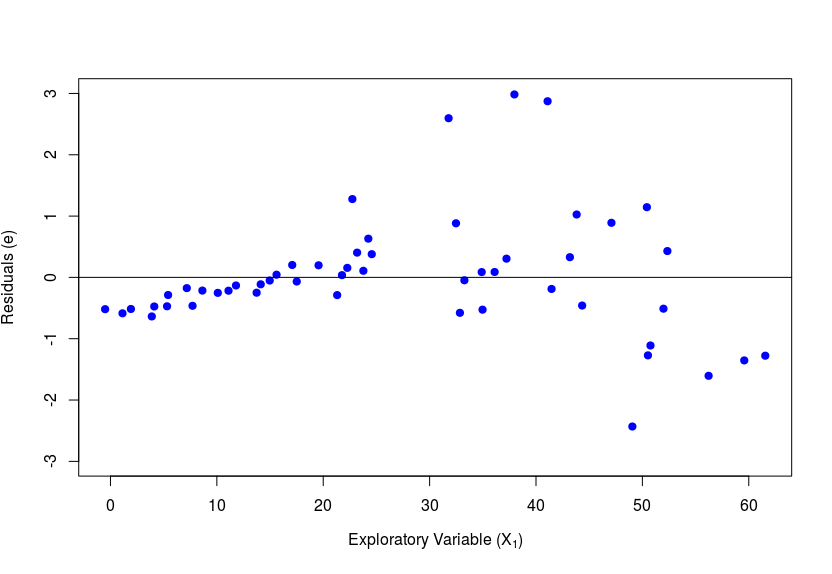
Also known by the term Homoscedasticity, this refers to the fact that the residual $e_i$ should have a near-constant variance when taken across all data points. In the graph below plot between $e_i$ and $\hat{y_i}$, the variance is low initially and increases later, which is a clear violation of this assumption. A detailed check would involve plots of $\hat{y_i}$ vs each $X_i$ one-by-one, keeping other $X_i$ constant or at the same level. As example of violation seen through this plot would be as below.
Similar to the previous case, one could try to transform individual $X_i$ variables. Another way to overcome this issue is using weighted least squares for model fitting instead of ordinary least squares. Here, one could assign a lower weight to records that cause more variation.

3. Uncorrelated Error Terms

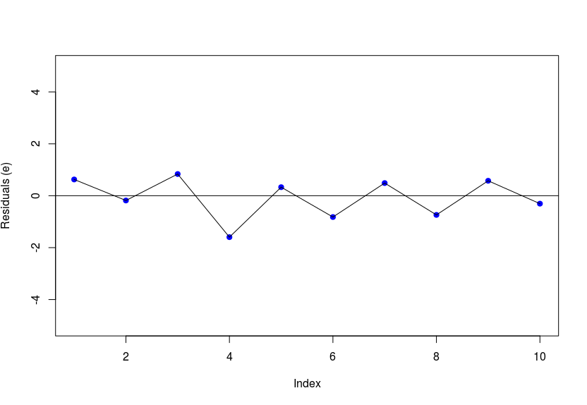
In a linear regression model, the error terms are assumed to be uncorrelated with each other. A plot of the residuals $e_i$ across data points should have no clear pattern. The graph below (zig-zag pattern) is a clear indication of negative correlation between residuals. However, it may not always be evident from the graph. A more scientific approach is to determine the Durbin–Watson statistic which is calculated as $DW = \frac{\sum_{i=1}^N (e_i-e_{i-1})^2}{\sum_{i=1}^N (e_i)^2}$, where N stands for the number of data records. A DW-stat value between 1 and 3 is ideal - the assumption is not violated. However, a value > 3 indicates negative correlation and a value < 1 means there exists positive correlation. This is a very difficult problem to correct if encountered. The use of generalized least squares instead of ordinary least squares for coefficient estimation could alleviate this issue to some extent.

4. No Outliers

The presence of outliers in the data can have an impact on the model because it gives a wrong picture of the actual relationship. The slope and intercept (coefficients) may be very different with and without outliers. The quality of the fit measured by $R^2$ also gets affected.
Ideally, it is best to get rid out outliers with the help of boxplots or other methods in the data preparation stage itself. One could also look at how much the outliers impact the model (the coefficients, $R^2$ ). This could be done by fitting the model with and without the outliers. Additionally, one can use Robust Standard Errors while checking for coefficient significance. This would take into account the fact there are outliers present in the data. The robust standard errors can also be used where we observe that the error terms do not have a constant variance (known as heteroscedasticity).

5. Normal Distribution of Error

The linear regression model requires that the residuals ($e_i$) follow a normal distribution with mean zero. If the cumulative distribution curve of the residuals follow a S-shape (as that of a standard normal CDF) or the probability density function (PDF) is approximately bell-shaped. However, it may become difficult to distinguish visually. In such a case, it is recommended that you perform a goodness-of-fit test that compares the observed v/s the theoretical values. One could go for either of the Chi-squared test or the K-S test.
In case of a violation of this assumption, one could try a variable transformation. For example, $X_i$ may not give normally distributed errors, instead one could try $\log{X_i}$. In the worst case, you may be required to switch to some other coefficient estimation technique like maximum likelihood estimation (rather than least squares method).

6. Absence of Multi-collinearity

If the absolute value of the correlation between two explanatory variables $|corr(X_1, X_2)|$ is greater than a threshold (usually 0.4 or 0.5), then it may result in multi-collinearity. In linear regression, it is assumed that the explanatory variables are independent of each other. A second level check for multi-collinearity could be done using the variation inflation factor (VIF). For this, you will need to build a linear regression model with one of the $X_i$ as dependent variable regressed with the other $X_i$ as the predictor variables. I’ll give you an example to make things clear. If we originally have 3 explanatory variables $X_1, X_2, X_3$ and you suspect that there is multi-collinearity, then you build a new regression model of the form $X_1=\beta_0+\beta_1X_2+\beta_2X_3$, and estimate the $R^2$. With this value of $R^2$, you can calculate the $VIF = \frac{1}{1-R^2}$. If the $VIF>10$, then one can conclude the presence of multi-collinearity, which is undesirable. One solution would be to drop one or more of the predictor variables $X_i$ and re-fit the model. The extend of correlation may decrease on doing some transformations. For example, use $\log{X_1}, \log{X_2}$ instead of $X_1, X_2$ .

So those were the assumptions that you need to consider when using linear regression to model your data. The consequences of violation can be anything ranging from a poor model fit to discarding variables from the model that were actually significant. The next time you use a linear regression model, make it a point to check whether these assumptions hold, if not, try out some of the remedial measures mentioned. This could ultimately lead to better model performance and would help in more accurate interpretation of the coefficients.

---