Text Classification using LSTM Networks - Dive Into Analytics Blog

It has been almost a year since I posted on my blog. I have been quite busy with my research work. In the past few months, I had the opportunity to gain some hands-on experience with deep learning. Looking at the number of papers that get published every week, there is no doubt that this is the right time to get into this field and work on some interesting problems. I have been working on some deep learning applications to NLP and on the way, I had the chance to familiarize myself with libraries such as Keras and Tensorflow. Enough of where I have been all this while, lets dive into the tutorial!

Sentiment Analysis

According to wikipedia, the aim of sentiment analysis is to determine the attitude of a speaker or writer towards a topic. Consumers usually tend to have opinions about products or services that they use, which they usually express through user reviews. Users can speak good about the product or may say that they were totally disappointed by the services offered. Now a product manager can go through all reviews and get an overall idea of how users feel about the product. Wouldn’t it be much more convenient if your machine learning algorithm can automate this process? That is, it goes through all the reviews and gives you a final score for the product. One can do more complicated things like identifying certain aspects of the products that the users liked/disliked - this is called Aspect Based Sentiment Analysis.

Long Short Term Memory Networks

Traditional neural networks are not suited to handle sequence data since they are unable to do reasoning based on previous events. Recurrent neural networks (RNN) tackle this issue by ‘remembering’ information from the previous time steps. The vanilla RNNs are rarely used because they suffer from the vangishing/exploding gradient problem. LSTMs or Long Short Term Memory Networks address this problem and are able to better handle ‘long-term dependencies’ by maintaining something called the cell state. The inflow and outflow of information to the cell state is contolled by three gating mechanisms, namely input gate, output gate and forget gate. I will not be going into the equations and mathematical details of LSTMs. If you are interested, the blog posts by Chris Olah and Andrej Karpathy.

Hands-On

Moving on to the actual code, I have used Keras to implement this project. First, I shall implement a very simple network with just 3 layers - an Embedding Layer, an LSTM layer and an output layer with a sigmoid activation function. I later modify the network and provide some tips that can be useful in order to achieve a better performance. You can find the Jupyter notebook on my Github. Here, I will be explaining only the important snippets of code.

Keras

Keras is a very high level framework for implementing deep neural networks in Python. It is build on top on frameworks such as Tensorflow, Theano and CNTK. One can use any of the three as the backend while writing Keras code. Keras is convenient to build simple networks in the sense that it involves just writing code for blocks of the neural network and connecting them together from start to end.

Dataset

The Rotten Tomatoes movie review dataset originally released by Pang and Lee, is a benchmark dataset in the area of sentiment analysis. It consists of about 11,000 sentences, half of which have a positive label and the other half have a negative label. The dataset can be downloaded from this link.

Data Pre-processing

In this section, we load the data from text files and create a pandas dataframe. We also make use of pre-trained word embeddings. Word embeddings are one of the ways to represent words as vectors. These vectors are obtained in a way that captures distributional semantics of words, that is, words that have a similar meaning or occur in a similar context tend to have a similar representation and hence would be closer to each other in the vector space. You can read this article for a better understanding of word embeddings. GloVe and word2vec are the most popular word embeddings used in the literature. I will use 300d word2vec embeddings trained on the Google news corpus in this project, and it can be downloaded here.

# Read the text files of positive and negative sentences
with open(DATA_DIR+'rt-polarity.neg', 'r', errors='ignore') as f:
    neg = f.readlines()
    
with open(DATA_DIR+'rt-polarity.pos', 'r', errors='ignore') as f:
    pos = f.readlines()

print('Number of negative sentences:', len(neg))
print('Number of positive sentences:', len(pos))

# Create a dataframe to store the sentence and polarity as 2 columns
df = pd.DataFrame(columns=['sentence', 'polarity'])
df['sentence'] = neg + pos
df['polarity'] = [0]*len(neg) + [1]*len(pos)
df = df.sample(frac=1, random_state=10) # Shuffle the rows
df.reset_index(inplace=True, drop=True)

The text data needs to be pre-processed into a sequence of numbers to be fed into a neural network. At this point, we need to assign an numerical index to each word in our corpus. But it may not always be possible to consider each and every word in our corpus. So we limit our vocabulary size to a maximum value (say 20,000), i.e., we consider only the most frequently occuring 20,000 words from the corpus. The remaining words can be replaced with a token. In our case, as you would see in the code snippet below, the number of distinct words is below the vocabulary limit.

Sentences in the dataset may be of varying lengths (number of words). However, we need to provide a fixed size input to the model. So the next decision that needs to be made is what sentence length would be ideal. Choosing a low value, say first 10 words of each sentence, we are able to reduce the computational compexity but at the cost of losing out some information (that might have been useful in classifying the polarity of the sentence). Analyzing the sentences, we find that 90 percentile of the sentences have atmost 31 words. In my case, I decide to pick 30 as the maximum sequence length. So sentences longer than 30 words with be truncated, and the shorter sentences will be zero padded.

To illustrate the concepts described above, imagine that my maximum sequence limit is sequence length is set to 10. An I have the following sentence: ‘The movie was totally WORTHLESS!’. First, I would remove all puctuations and convert the words to lower case, then covert the sentence into a list of words. The words are then replaced by their corresponding indices by looking up a dictionary. The final step is to pad/truncate the sequence. Since the maximum sequence length is 10, the list is expanded to that size by filling in with zero values.

Word Tokenize:  ['the', 'movie', 'was', 'totally', 'worthless']
Index Sequence: [1, 12, 4, 245, 358]
Zero Padding:   [1, 12, 4, 245, 358, 0, 0, 0, 0, 0]

The way all of the above is done in keras is pretty simple:

# Pre-processing involves removal of puctuations and converting text to lower case
word_seq = [text_to_word_sequence(sent) for sent in df['sentence']]
print('90th Percentile Sentence Length:', np.percentile([len(seq) for seq in word_seq], 90)) # Output: 31

tokenizer = Tokenizer(num_words=MAX_VOCAB_SIZE)
tokenizer.fit_on_texts([' '.join(seq[:MAX_SENT_LEN]) for seq in word_seq])

print("Number of words in vocabulary:", len(tokenizer.word_index)) # Output: 19180

# Convert the sequence of words to sequnce of indices
X = tokenizer.texts_to_sequences([' '.join(seq[:MAX_SENT_LEN]) for seq in word_seq])
X = pad_sequences(X, maxlen=MAX_SENT_LEN, padding='post', truncating='post')

y = df['polarity']

X_train, X_test, y_train, y_test = train_test_split(X, y, random_state=10, test_size=0.1)

The last line in the snippet above just splits the data into training and validation sets using the functionality from sklearn. Next we load the embeddings and create an embedding look up matrix as follows. With the help of this matrix, for any given word in our vocabulary, we would be able to lookup the 300d embedding vector or that word. In case, the word is not present in the pre-trained list of embeddings, then we use a randomly initialized vector of 300-dimension.

# Load the word2vec embeddings 
embeddings = gensim.models.KeyedVectors.load_word2vec_format(W2V_DIR, binary=True)

# Create an embedding matrix containing only the word's in our vocabulary
# If the word does not have a pre-trained embedding, then randomly initialize the embedding
embeddings_matrix = np.random.uniform(-0.05, 0.05, size=(len(tokenizer.word_index)+1, EMBEDDING_DIM)) # +1 is because the matrix indices start with 0
for word, i in tokenizer.word_index.items(): # i=0 is the embedding for the zero padding
    try:
        embeddings_vector = embeddings[word]
    except KeyError:
        embeddings_vector = None
    if embeddings_vector is not None:
        embeddings_matrix[i] = embeddings_vector
        
del embeddings

Finally, we have all the data ready and move on to the model building part. In this example, we use the Sequential Modelling API from Keras. In this framework, we basically define layers and stack them one over the other in a sequential manner. The other API is the Functional API, which we will keep it for some other day.

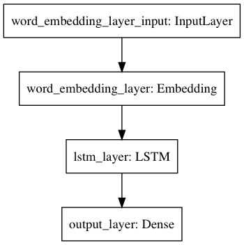
# Build a sequential model by stacking neural net units 
model = Sequential()
model.add(Embedding(input_dim=len(tokenizer.word_index)+1,
                          output_dim=EMBEDDING_DIM,
                          weights = [embeddings_matrix], trainable=False, name='word_embedding_layer', 
                          mask_zero=True))

model.add(LSTM(LSTM_DIM, return_sequences=False, name='lstm_layer'))

model.add(Dense(1, activation='sigmoid', name='output_layer'))

The first layer is an Embedding layer, which takes as input a sequence of integer indices and returns a matrix of word embeddings. The next layer is an LSTM which processes the sequence of word vectors. Here, the output of the LSTM network is 128-dimensional vector which is fed into a dense network with a sigmoid activation in order to output a probability value. This probability can then be rounded off to get the predicted class label, 0 or 1. The model.summary() function is useful to verify the model in terms of what goes as inputs and outputs and what are the shaped of those. We also get an idea of the number of parameters that the model has to train and optimize. In this case, the non-trainable parameters are the word-embeddings.

_________________________________________________________________
Layer (type)                 Output Shape              Param    
=================================================================
word_embedding_layer (Embedd (None, None, 300)         5754300   
_________________________________________________________________
lstm_layer (LSTM)            (None, 128)               219648    
_________________________________________________________________
output_layer (Dense)         (None, 1)                 129       
=================================================================
Total params: 5,974,077
Trainable params: 219,777
Non-trainable params: 5,754,300
_________________________________________________________________

One can also get a visual feel of the model by using the plot_model utility in Keras.

The last steps are pretty simple. The model needs to be compiled before actually training. Here, we need to specify the loss function, the optimizer and the metrics that needs to be monitored throughout the training. The training process will begin once the model.fit() is called. The arguments to this function include the number of epochs of training, batch size and the training and validation sets. One epoch refers to one run through the entire training dataset. The training data is split into batches and the model parameters are updated after each batch is processed.

model.compile(loss='binary_crossentropy',
              optimizer='adam',
              metrics=['accuracy'])

model.fit(X_train, y_train,
          batch_size=BATCH_SIZE,
          epochs=N_EPOCHS,
          validation_data=(X_test, y_test))

score, acc = model.evaluate(X_test, y_test,
                            batch_size=BATCH_SIZE)

print("Accuracy on Test Set = {0:4.3f}".format(acc))

On evaluating the model, I get an accuracy of 80.4%, which is decent considering the fact the the network that I used is pretty rudimentary.

Next, lets try modifying the network above with the following tricks, in the hope of achieving a better performance:

Bi-directional LSTM: The LSTM that I used reads the sequence in the forward direction, i.e., from the first word to the last word. We can try reading the sentence in a reverse fashion as well (which has been proven to do well in tasks such as POS tagging). In the bidirectional LSTM, the final hidden states of the foward and the backward LSTMs are concatenated and passed on to the downstream network.
Batch-normalization: This is a method introduced by Ioffe & Szegedy, that helps speed up the training process and simultaneously reduce over-fitting. To prevent instability of the network during training, we usually normalize the inputs to the model by subtract the mean value and dividing by the standard deviation. With batch-normalization, the output of a previous layer is normalized in the same manner, before it is fed into the next layer. For feed-forward networks, batch-normalization is carried out before applying the activation function.
Dropout: A simple yet powerful regularization technique, that states that some nodes in the network can be ignored during some iterations of training. That is, a given node will participate in the forward and backward pass (weight update), with the desired keep probability (which is 1.0 - dropout_probability). The idea is that during training, the network learns to predict using only a subset of the weights. This would intuitively mean that during test time, when it can use the entire set of weights, it should have a better predicting power.
Trainable Embeddings: In the basic model, the pre-trained word embeddings were used as is. However, we have an option to allow even the word embeddings to be trainable parameters, i.e., they embeddings are adjusted during the gradient descent procedure. One needs to be aware that setting trainable=True can result in the word embeddings tuned to overfit on the training data and perform poorly on the validation set.

The code has been posted on my Github. The accuracy increased to 81.5%, the performance improvement was not as much as I expected inspite of a more complicated network. If you are interested, you can play around with some of these parameters and see its effect on validation accuracy.

This was a simple post that demonstrated the use of LSTMs for text classification. Sentiment analysis has been a widely explored problem - if you go beyond the usual sentences, you would need to handle issues such as negation and sarcasm in sentences. You could formulate this as a regression problem and obtain a score rather than outputting a class label. As for LSTMs, they are powerful and have been utilized in a wide variety of NLP tasks. I will be back with more deep learning stuff in my future blog posts.

← Previous Post