Kaggle Seizure Prediction Competition

I happened to participate in a Kaggle Competition as a project for my course on Statistical Learning at the University of Waterloo. So Kaggle is a platform where organizations can host data science competitions, most of which have good prize money for the winners. Anyone can register and participate, and most of these competitions are extremely challenging because you are competing against the top data scientists around the world. However, this was an amazing learning experience for me and now that the competition has ended, I wish to share my modelling approach through this post.

Introduction

Epilepsy is a brain disorder that affects 1% of the world’s population. Individuals with epilepsy are prone to seizures from time to time. With the recent availability of data from sensors like EEG, that record electrical activity of the brain, scientists are now using data driven approaches to predict the onset of seizures. If accurate predictions can be made, the patient can be warned in advance so that he/she can take the necessary precautions.

Problem Statement and Data

The competition was hosted by the University of Melbourne who had provided data from 3 patients. For each patient, iEEG signal recordings from 16 electrodes were sampled at 400Hz and the data was in the form of 10-min interval files.

The state of the brain can be generally classified into four:

1. Inter-ictal (normal state or baseline)
2. Pre-ictal (just before the seizure)
3. Ictal (during seizure)
4. Post-ictal (just after seizure)

The data provided for this competition had interictal clips (restricted to be at least four hours before or after any seizure) and pre-ictal clips (one hour prior to seizure). The goal is to classify these 10 minute clips into either interictal or pre-ictal. Each 10-min file had 240,000 readings. There were 3 sets of files, one for each patient, totalling to over 50 GB of data. The training set data had the labels pre-specified. The participants were required to predict and submit labels/probabilities for the test set records for each patient. The evaluation criteria was the area under the receiver-operater characteristics (ROC) curve, better known as AUC. The higher the AUC, the better the prediction.

Data Pre-Processing

Prior to data modelling, it is always a good idea to do some pre-processing. The .mat files provided had 240,000 readings per file. In order to reduce computational complexity and to represent the data in a compact format, a signal processing technique called resampling was used. Essentially, every sequence of 400 readings was compressed into 1 data point, which makes it 1 reading per second, a total of 600 readings per file. Shown below is a sample EEG reading file before and after resampling. As can be seen, the overall trends in the signal is captured while the noise is eliminated.

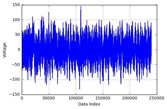Figure: Voltage Fluctuations in the original file 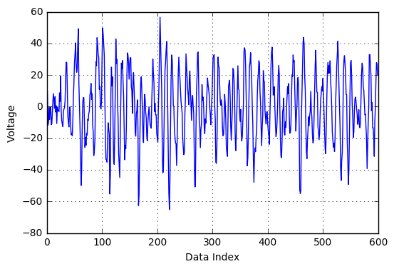Figure: Voltage Fluctuations in the resample file

Feature Extraction

Feature Engineering is a very important step in any machine learning application. Spending a good amount of time to choose the right set of features will be fruitful in giving good predictions later. In this study, the following features were used for training and fitting the boosting algorithm, which are classified into 3 categories:

Time Domain Features

For each of the 16 channel time series, 4 statistical measures were extracted:

1. Minimum EEG reading
2. Maximum EEG reading
3. Variance
4. Kurtosis, the fourth statistical moment

Two other features extracted in the time domain after some matrix algebra on the data are as follows:

1. The highest 3 singular values obtained after Singular Value Decomposition of the resampled 600x16 data matrix
2. Highest eigenvalue of the 16x16 Pearson Correlation Matrix between the channels

Frequency Domain Features

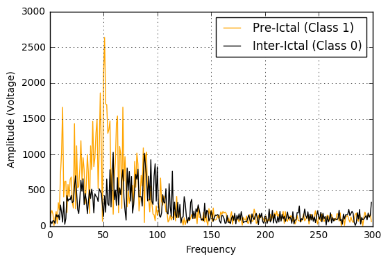
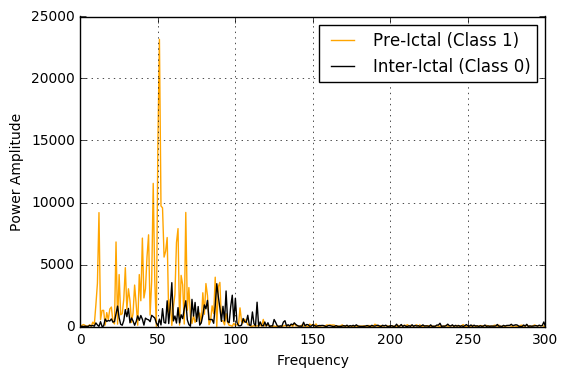
Applying a Fourier Transform to the signal is required to extract the features in this category. The Fourier Transform is a method to decompose a waveform as a sum of multiple sine and cosine functions. Representing the signal in the frequency domain gives an idea of which frequencies have the highest energy. The features extracted were:

1. Highest amplitude of the signal in the frequency domain
2. The power of the signal at different frequencies were obtained from the periodogram. The maximum power was calculated at 4 different frequency bands: (i) Delta: 0-4 Hz (ii) Theta: 4-8 Hz (iii) Alpha: 8-12 Hz (iv) Beta: 12-30 Hz

As can be seen in the figures below, the pre-ictals tend to have a much higher power amplitude as well voltage amplitude when analyzed in the frequency domain. Hence, these would indeed be distinguishing features in this classification problem.

EEG Specific Features

The next set features we choose are the ones that have been reported in the literature to be helpful in classifying EEG data:

1. Spectral Entropy: This is a measure of uncertainty or randomness in the signal. Preictal time series are seen to be more disorderly than the usual interictals.
2. Hurst Exponent (H): A high value of Hurst exponent (0.5 < H < 1) indicates that the signal frequently switches between high and low voltages, whereas a low value (0 < H <= 0.5) shows that the time series hovers just around the mean value.
3. Higuchi Fractal Dimension (HFD): This feature has been shown to quantify the dimensional complexity of a times series. The EEG readings just before the onset of seizure would be more complex to represent, than the one during the normal activity of the brain.

Model Fitting

From the 3 categories of features described in the previous section, we now have 196 features available for training. For carrying out the classification task, the XGB implementation of the boosting algorithm was used. Boosting is an additive and iterative tree-based supervised machine learning approach, where we construct a strong classifier from multiple weak learners. In order to avoid over-fitting, 5-fold cross-validation was carried out with stratified sampling (which ensures the class ratio of 0s and 1s in the training sets were representative of the data). The parameters of the model were tuned to obtain an AUC of 0.67 on our validation set. The parameters used were :

1. n_estimators = 500: Refers to the number of trees to be grown to fit the model.
2. max_depth = 9: Number of splits for each of the weak learner trees.
3. learning_rate = 0.1: This is the shrinkage parameter that slows down the learning rate while achieving higher accuracy.
4. sub_sample = 0.8; Each tree uses a random subset of size 80% of the original.

Model Enhancement

When the predicted probabilities from the XGB model discussed in the previous section was submitted to Kaggle, after running it on the actual test set, the AUC wasn’t that great! So we dug deep to understand what might have caused the model to perform poorly. We came up with 2 issues in the data that required to be tackled in order to improve the AUC score.

1. The first issue was as a result of the highly skewed and imbalanced dataset. The number of records were in the proportion 7% Class-1 (Pre-ictal) and 93% Class-0 (Inter-ictal). In order to accurately fit the model, we initially started with the idea of undersampling - randomly sampling a fraction of the records of the majority class. However, this meant that we were not making use of entire training set. So an oversampling techinque called SMOTE (Synthetic Minority Oversampling Technique) was adopted. Essentially, this method introduces synthetic samples in the neighborhood of each data point from the minority class. The feature values of these synthetic observations are calculated based on the feature values of the original minority class records in their respective neighborhood. By oversampling the minority class, we now have equal proportions of data points from both classes for training.
   
2. The second issue was that there existed strong correlation between the features that we had extracted. This challenge was overcome with the use of Principal Component Analysis (PCA). PCA is capable of capturing strong patterns in the data and the derived components are linear combination of the original features. Applying this data transformation technique, we extracted independent components in the directions of maximum variation. The number of components was set to 25 based on tuning to maximize AUC. If you are further interested in understanding PCA, I highly recommend this blog post, which explains the concept with awesome visualizations.

Results and Conclusions

The AUC on our cross-validation set improved from 0.67 to 0.75 by incorporating PCA and SMOTE to the original model. And, the AUC on the Kaggle test set with the boosting model was around 0.69 - Not the best, but a good point to start with. Since the dataset provided was huge, the data pre-processing indeed plays a big role. We did not properly handle the issues occuring from data dropout (the EEG electrodes do not make any measurements during some time intervals and as a result all readings become zero for that interval). Feature selection also becomes a challenging task in such competitions. With a better understanding of signal processing and if more computational power is available, one could explore and identify more useful features.

So obviously, we did not win the competition, but this being my first Kaggle competition, it was a good learning experience. Sorry if this post was way too technical! If anyone is interested in playing around with the code, tuning the model parameters and making submissions to Kaggle, I have shared my code as an IPython notebook on my github repository .

---